
Modified: July 14, 2025
Posted: July 14, 2025
This directory contains jpg images of scans of the 1400 MHz contimuum strip chart record covering roughly one day following the Wow! Signal occurrence.
The data starts on August 16, 1977 at 06h 20m LMST (at the longitude of the OSURO), and ends on August 17, 1977 at 07h 40M LMST. The declination of observation (the true declination observed) is -27d 00m.
You can download all images in this zip file archive:
http://naapo.org/~rchilders/lobes_data/misc/continuum_scans/Photos-1-001.zip. Alternatively,
each of the jpeg images is unpacked and is accessible at the directory link above.
Each scan covers one sidereal hour. The start of the following sidereal hour is written by hand in blue on the right-hand side of the folded-out page. The 5K noise tube fires for 5 solar minutes every 2 solar hours. There may be a 3-second rise time, as indicated in the hand-written notations. This would give an idea of the time constant of the continuum receiver system. When the strip chart would go off-scale, the pen retraced to the "top" of the chart to prevent flat-lining. The noise tube signal was injected into the "trailing" feedhorn, which is the second feedhorn a source image would pass through in drift scan survey mode. It is left as an exercise for researchers to determine when the noise tube fires with respect to the top of the local solar clock.
The system seems to have had low sensitivity, even for a 3-second time constant. There are many faint radio sources which are not evident. However, the glactic plane / galactic center is apparent at 17h 50m LMST, and other point sources at 21h 15m, 20h 39m (during an unexplained 10-minute duration noise tube), 19h 10m, 18h 58m, 16h 27m, 13h 47m, 01h 16m, and 01h 37m LMST.
Posted: August 15, 2023
This directory contains folders which contain png images of scans of old OSURO / Big Ear 50-channel (10 kHz narrowband channels) paper output.
An interesting folder is this one, which contains images around the time of the WOW signal (August 15, 1977).
You can access all archived data here
Posted: March 20, 2023
This file: OSS.txt contains a table of all Ohio Sky Survey point sources detected at 1415 MHz. The table is sorted by the catalog identifier, which corresponds to the right ascension of each source. The right ascension and declination of each source has been precessed to Julian 1950.0 epoch, to allow for a common coordinate system for radio sources observed at different calendar dates. The columns in OSS.txt are:
Catalog ID
Right Ascension (J1950.0)
Declination (J1950.0)
1950.0 = Julian epoch
1415 = Center frequency of radio receiver
Flux unit of source at 1415 MHz
Secondary catalog ID
Column 1 has a scheme for all sources, based on the right ascension (J1950.0) in which it was observed. The first character is always a capital "O" to indicate it is an Ohio Sky Survey catalog identifier. The second character is a B through Z, excluding "O":
1st/2nd character  Right Ascension hour (J1950.0)
-----------------  ------------------------------
       OB                       00
       OC                       01
       OD                       02
       OE                       03
       OF                       04
       OG                       05
       OH                       06
       OI                       07
       OJ                       08
       OK                       09
       OL                       10
       OM                       11
       ON                       12
       OP                       13
       OQ                       14
       OR                       15
       OS                       16
       OT                       17
       OU                       18
       OV                       19
       OW                       20
       OX                       21
       OY                       22
       OZ                       23
Posted: February 16, 2020
Here is a pdf of the presentation conducted by Bob Dixon and Russ Childers on February 13, 2020. It presents the history of the Ohio Argus Array, its current hardware, software, technical aspects, and some interesting observations. Click here: Presentation
Posted: November 24, 2019
Here are the unix commands to download/check the raw continuum data, log files, and programs. This data was collected concurrent with the LOBES (Low Budget ETI Search) survey, and so sometimes the feedhorns were moving (so LOBES could follow up on interesting narrowband sources).
Get the continuum data and put it into a local directory "RO-LOBES-Cont":
wget -r -np -nH -R "index.html*" --cut-dirs=2 http://ohioargus.org/~rchilders/contin/RO-LOBES-Cont/
Check the data with a checksum:
cd RO-LOBES-Cont
sha256sum -c OSURO_CONTIN_SHA256SUM
Get the narrowband LOBES data and put it into a directory "lobes_data":
wget -r -np -nH -R "index.html*" --cut-dirs=1 http://naapo.org/~rchilders/lobes_data/
Check the data with a checksum:
cd lobes_data
sha256sum -c LOBES_SHA256SUM
Posted: February 19, 2017
In the 1990s, while I was conducting the LOBES all-sky survey at the OSURO, the LOBES system detected a narrowband stellar source and moved the feedhorns to track it. After I made excited correspondences with Bob Dixon, he suggested that it sounded like a hydroxyl (OH) maser at 1612 MHz. Sure enough, after some research it turns out that the OSURO saw an extremely strong OH maser close to the galactic plane in the vicinity of the Cygnus X-ray source. Below is the catalog which I used to look up the source. The source of the maser is a red hypergiant star known as "NML Cygni" or "NML CYG". The frequency LOBES detected was 1612.231 MHz (or so); the declination of the beams was +40 degrees 00 minutes; the Right Ascension was around 20h 46m (Local Mean Sidereal Time).
A catalogue of stellar 1612 MHz maser sources
Even though this was not an artificial radio source, it does provide a very good test point in the sky for calibration (or reality checks or first light) for narrowband radio astronomy equipment. In fact, here is someone who did just that:
Posted: December 12, 2015
Here is a basic flowchart of the Ohio Argus array. Each of the "Linux Workstations" is dedicated to analying the snapshots of data taken from the DDCs, as packetized and sent via UDP from the Win98 Control PC Workstation.
Click on the image for a higher resolution image.
Posted: September 19, 2013
The USNO provides handy web pages for you to determine the rise and set times of the Sun and Moon (and other celestial objects) at this page.
For instance, you can get the position of the Sun and moon, in altitude/azimuth coordinates at 10-minute intervals from the first link at that page: Complete Sun and Moon Data for One Day. One aspect of this page of particular interest is that you can tell where the Moon will rise (the azimuth when the altitude is low), and so you can plan your foreground location if you want to do any lunar photography.
One can automate the above web page for a daily real-time display of where the Sun and Moon are right now (for pointing a telescope, for example), without doing a lot of calculations yourself. Here's a clue how:
This link
will return a table of the Sun's alt/az for September 19, 2013 for Columbus, OH (alt>=-12 degrees). Times are in EDT.
Codes:
USA city: FFX=1; Latitude/longitude: FFX=2; Sun: obj=10; Moon: obj=11; xxy: year=2013; xxm: month=9; xxd: day=19;
xxi: minute interval=10; st: state=OH; place: city=columbus; ZZZ: end-of-form=END
Posted: February 15, 2013
I've added a couple of real-time diagnostic pages so anyone can see the condition of Argus elements. They are links from: https://ohioargus.org/displays.html
1) I wanted to see if there was local radio frequency interference (RFI),
and I wanted to see if elements were seeing the Sun, so I created a page
which does interferometry between the "reference element" and the rest
of the elements:
https://ohioargus.org/Argus/data/fringe_lasthour.html
This data is plotted for the entire day, starting from 0 hours UTC.
The x-axis is "seconds from 0 hours UTC, and the y-axis is the mean of the product
of the in-phase samples of each element times the "reference element". Data is
averaged over 480 sets of 16384 antenna snapshots (8 minutes). If there is
no (strong) interference, and if there are no (strong)
sources in the sky, then the output from each element should be uncorrelated
with the other elements, and each plot should hug the x-axis (y=0) in all plots.
If there is constant interference, then there would be constant offset.
If there is a strong, moving source (eg the Sun), then the correlations move
smoothly from positive, through zero, to negative.
What might cause local interference?
* experiments in the saucer field
* electrical equipment in the SatComm facility
* antenna towers broadcasting microwave signals
* cross-coupling between antenna amplifiers
2) Each element in the array should be a clone of every other, providing
identical frequency response; identical responses to the calibration noise
source; and identical noise floor. I've been looking at these data on and
off for years, but only now decided to plot them in so they are accessible
to everyone:
https://ohioargus.org/Argus/data/power_lasthour.html
This data is plotted for the last 2 hours. The x-axis is "seconds since
0 hours UTC", and the y-axis is "power in decibels". There should be two
straight lines in each plot - a top line for when the calibration noise
source is "on" (1 out of 60 seconds), and a bottom for when the noise
source is off (59 out of 60 seconds). As one can see, these lines are
rarely straight, and some are misbehaving badly. There should be only 2
things which effect the lines - precipitation on the spiral antennas and
radio waves being impinging on the spiral antennas. And when there is
either one of these 2 conditions, EACH element should show the SAME effect.
What might cause differences between Argus elements?
* spiral antennas with dissimilar frequency response
* failing amplifiers in spiral antenna
* bad connecting cable between antenna and amplifier box
* failing 20dB amplifiers
* intermittent connection between 12v power supply and 20dB amplifiers
* intermittent connections in 100-foot cable between 20dB amplifiers and receivers
* failing components on receivers
* failing components on receiver backplanes
* failing receiver power supplies
* failing receiver local oscillator distribution
* failing connections between receivers and DDCs
* failing DDCs
* failing DDC backplanes
* failing DDC power supplies
* failing DDC "corner turner"
* failing ribbon cable between "corner turner" and digital I/O card
* failing digital I/O card
Note: I have worked on all of the above, since joining the Argus Array project in 2003. Most of the above are one-of-a-kind components, and their failure would mean that Argus would go off the air. Thus, any approach to address issues with these components requires great caution. The fact that there are so many points of failure also underscores the need to get a parallel Argus up and running, if it is desired to keep an observing program going.
Posted: November 9, 2009
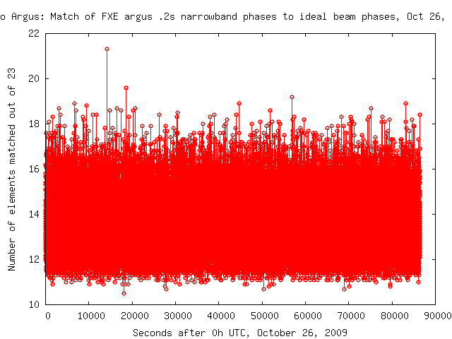
On October 26, 2009 at 3:57 UTC, Argus reported seeing a narrowband signal high in the sky, at 76 degrees altitude. The signal was not rejected as interference, because it made an excellent match to what a signal would look like if it were coming from far away. I have programmed Argus to store a 5-minute block of data including the signal when such good "match" events occur. Below is a plot of the matches at the time the signal appeared. The "signal" is the spike up to 21.5 "elements matched", at 14160 seconds after 0 hours UTC:
Argus emailed me that it saw something interesting, and once
I determined that it was unlikely to be interference or a phenomenon
associated with satellites, I downloaded the 5-minutes of data and
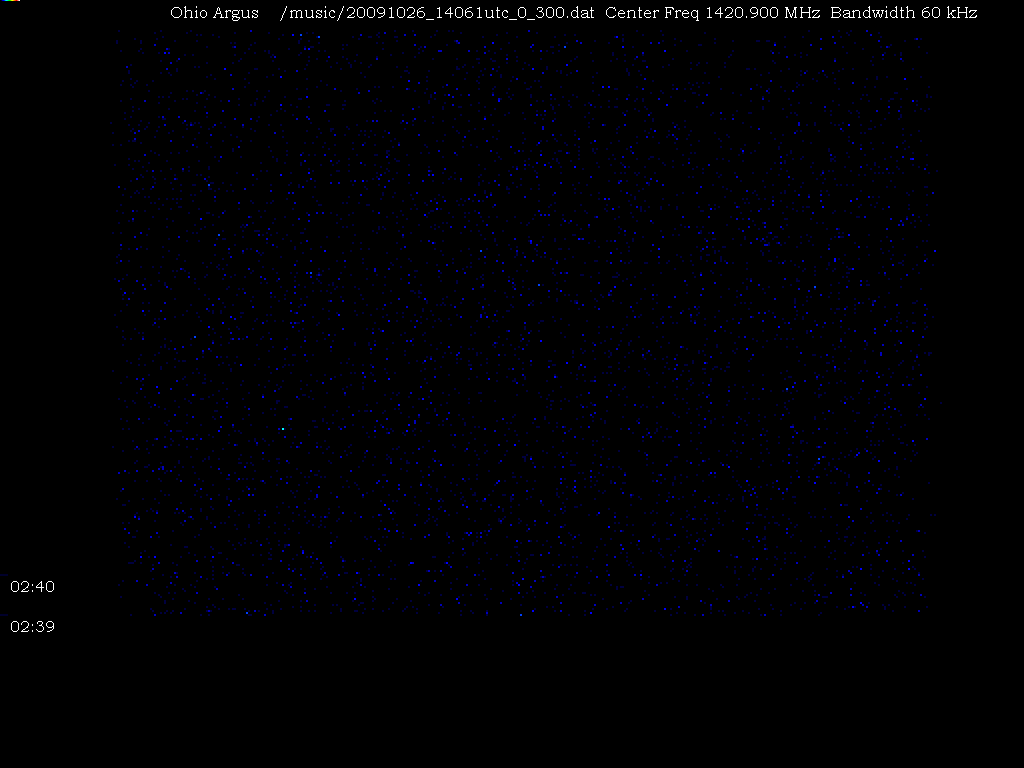
began the analysis. The first thing I did was use an offline
data analysis program to "point" a beam at the location of the
signal. Here is the resultant waterfall display. The center
frequency is 1420.900 MHz, and the bandwidth is 60 kHz. The
earliest data is at the bottom and the most recent is at the top.
There are 293 one-second acquisitions shown in this waterfall plot.
The signal shows up as the green dot in the lower left. (Ignore
the time on the left-hand margin):
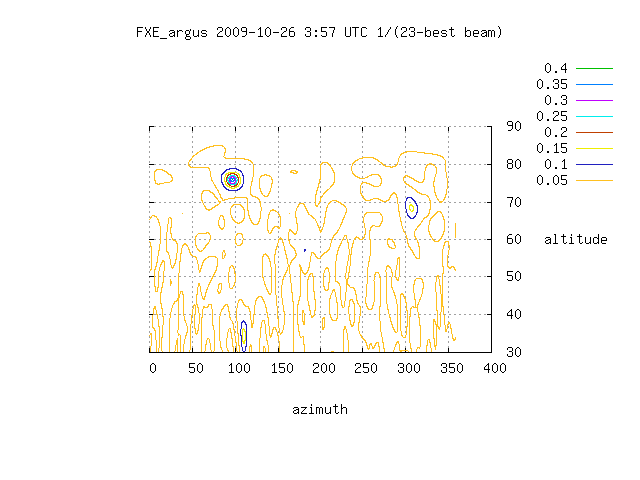
These matches rarely occur unless a real signal - like the sun or a
satellite - is really out there. This is what gets me excited
about this signal. These signals with a good match to an ideal
beam also make nice sky maps. Here is a map of the "goodness of
fit" of the data to an ideal beam. The fit to the beam at altitude
76, azimuth 97 is the best one:
I have corresponded with Bob Dixon and Steve
Ellingson, and they gave me some good advice on how to show that
this was a real signal and not some statistical anomaly. They also
told me that it doesn't qualify yet as a true SETI signal
candidate, because it was observed only once, from one vantage
point, and not for a long
enough period to determine if it moves with the backdrop of stars.
Nonetheless, it is exciting to think that this may be a signal
from a planet around a star in the globular cluster NGC 752, a
mere 1,300 light years away. The signal coordinates are marked
by the crosshairs in the sky map below. The position may be off
by a few degrees due to uncertainty in the exact pointing of
the array, however NGC 752 falls within Argus's 5-degree half power
beam width (at 1420 MHz):
I am following up on Bob and Steve's suggestions. One thing that
would kick my excitement into high gear is if more activity is seen
in that same part of the sky. I have now dedicated an Argus beamforming
computer to tracking the signal location, and alerting me if any
activity is seen in that part of the sky again. I am also plowing
through all the frequency bins in the 5-minute archive to see if any
other weaker signals are in the data, but were missed.
For more information, see this URL: https://ohioargus.org/~rchilders/oct26_2009_strike/index_20091026.html
Posted: June 11, 2009
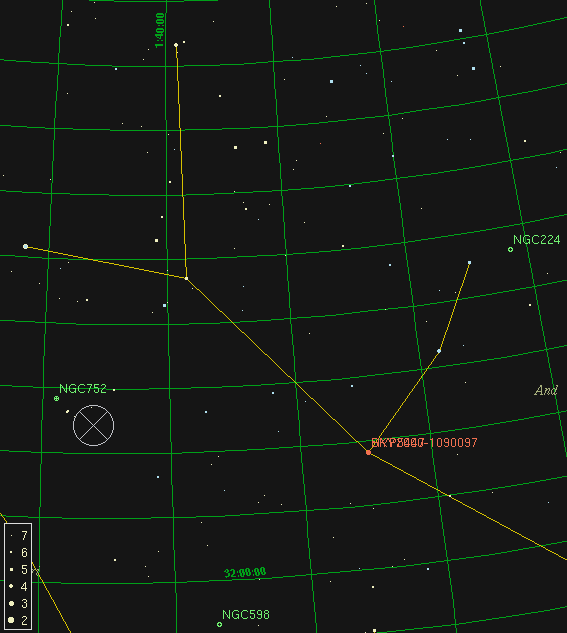
Until recently, the Ohio Argus array could only detect near-earth objects like satellites and airplanes, or the Sun. Now, with some tweaking, Argus is seeing the Cygnus Complex, which passes overhead in the Northern Hemisphere during the summer months. Cygnus, being at about +40 degrees declination, passes directly over Argus, which is at 40 degrees North latitude. See this image of the radio sky from Kraus's Radio Astronomy, and look for Cygnus at 20-21 hours Right Ascension, 35-50 degrees declination.
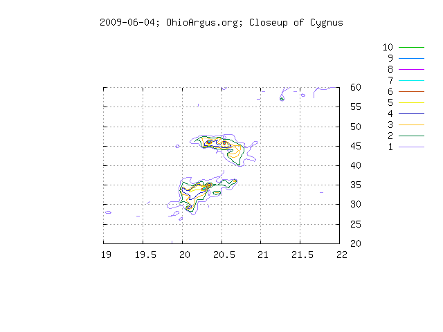
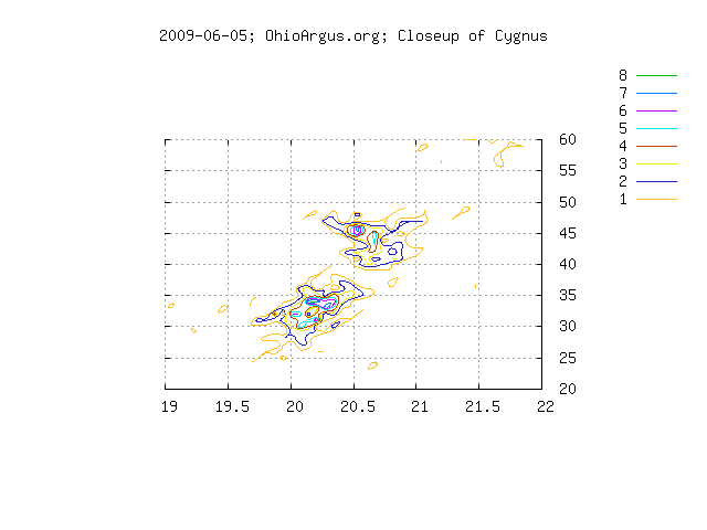
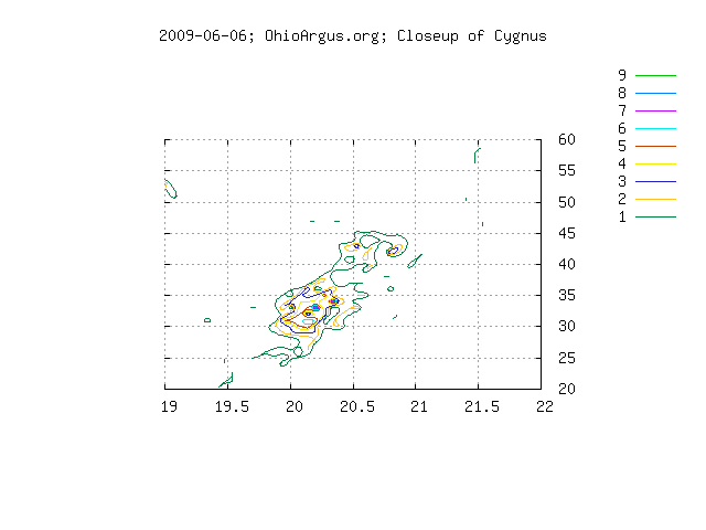
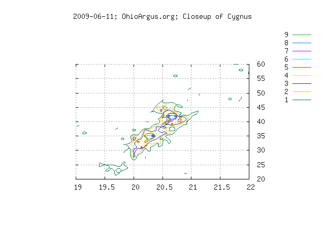
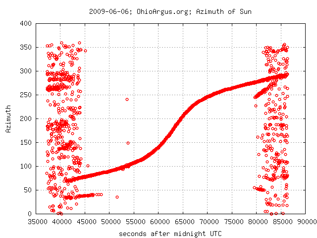
The above images show the Cygnus Complex as seen by Argus over 4 nights in June 2009. Note the bright spot at 20h 20m RA, 35 degrees dec. This is Cygnus X-1, I believe. Cygnus X-1 is actually closer to 20h 0m RA, but the error may be due to a calibration bias. There may be additional issues due to the fact that there is a lot of energy in the sky at 1420.500 MHz, and the beamformer which formed the above image was assuming that the brightest object is a point source. In addition to seeing Cygnus, the Sun is also (relatively) accurately positioned when it is above 20 degrees altitude. This cutoff used to be 30 degrees. Argus also is acting more like Jim Bolinger's array, which could locate weather stations on the horizon: now Argus can point at the azimuth of the sun when it is on the horizon.
The azimuth of the Sun on June 6, 2009:
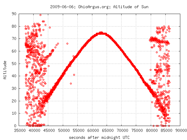
The altitude of the Sun on June 6, 2009:
So what did I do to improve the sensitivity of Argus? The LNAs and 20 dB amplifiers early in each element's receiver chain is powered by a 12 volt (DC) power supply. All I did was decrease the voltage down to 10 volts and the signal-to-noise ratio increased by 3 to 6 dB for each element. Apparently that extra 2 volts was amplifying "noise" more than it was "signal". Decreasing the voltage below 10 volts does not further increase sensitivity.
Turning down the voltage was just a guess on my part, but it was based on an experience I had at Big Ear. Chief Engineer Steve Brown and I were looking at how to increase the sensitivity of the LOBES (SETI) receiver/signal detector. We looked at the spectral output of the analog receivers and saw what we thought was "normal" noise, including some "birdies". However, when we attenuated the incoming Local Oscillator signal by 10 dB suddenly a lot of those birdies and noise vanished! Apparently the LO was so strong that it was "distorting" the spectrum.
One more thing I did to improve things was to replace the yagi calibration antenna and replace it with the dual-dipole antenna originally used on the Lonc 1420 MHz Signal Squirter. Argus uses the phase it sees at each element when the calibration source is on, to compare theoretical phase values (determined by the array geometry and the center frequency) with actual phase values. A yagi antenna changes phase in radical, unknown ways dependent on small variations in antenna construction. The dual-dipole changes phase very "slowly". At some point I would like to use a simple dipole as a calibration source, as its phase is much more "flat", for all receivers a given distance from the center of the dipole.
Thankfully, we now have an HP RF power meter, and so I was able to test the output powers of the yagi and dipole calibration antennas, and was also able to look at the output of elements, with their DC power at 12 volts, and at the lower-noise 10-volt level. Many thanks to NAAPO for approving the funds to purchase this critical piece of test equipment for the Ohio Argus array.
Each day's data file has a very easy pattern to recognize:

Here is the data for January 20, 2009:
https://ohioargus.org/~rchilders/mxe_20090120.txt
Here is the data for January 19, 2009:
https://ohioargus.org/~rchilders/mxe_20090119.txt
Here is the data for January 18, 2009:
https://ohioargus.org/~rchilders/mxe_20090118.txt

The name of the file is mxe_YYYYMMDD.txt, where YYYY is "year", MM is
"month", and "DD" is "day of month".  All numbers are padded with
leading zeros for days or months less than 10.  Data is taken once
every 10 seconds, so ideally there would be 8640 lines in the file.
Due to the time taken for calibration (once per minute) and other
factors, the number of lines is always less than 8640 per day.

The data in the files is text.  The data is in 9 columns:

1) The second-of-day UTC that the data was collected
2) Number of array snapshots analyzed (16384*10)
3) Always zero for "mxe" data
4) The "Power" of the "best source"
5) The Altitude of the "best source"
6) The Azimuth of the "best source"
7) The number of array element "phase matches" of the "best source"
8) The Right Ascension (in degrees) of the "best source "
9) The Declination of the "best source"

The "best source" is defined as the source whose phases are most like
an ideal beam at a particular alt/az.  The best source is NOT the
point in the sky with the highest power, because that could easily be
caused by local interference flooding the aperture.

There are also data files for 16384 array snapshots (txe) and data
files for narrow-band files (fxe).  I am not pulling those data files
down right now.  Maybe a hard drive can be added to a SatComm server
which will hold all these data files (or backups of these files).

So anyone can download the above files and analyze them in MATLAB or
Octave or R, or can build Unix scripts to parse the data and generate
images and animations.
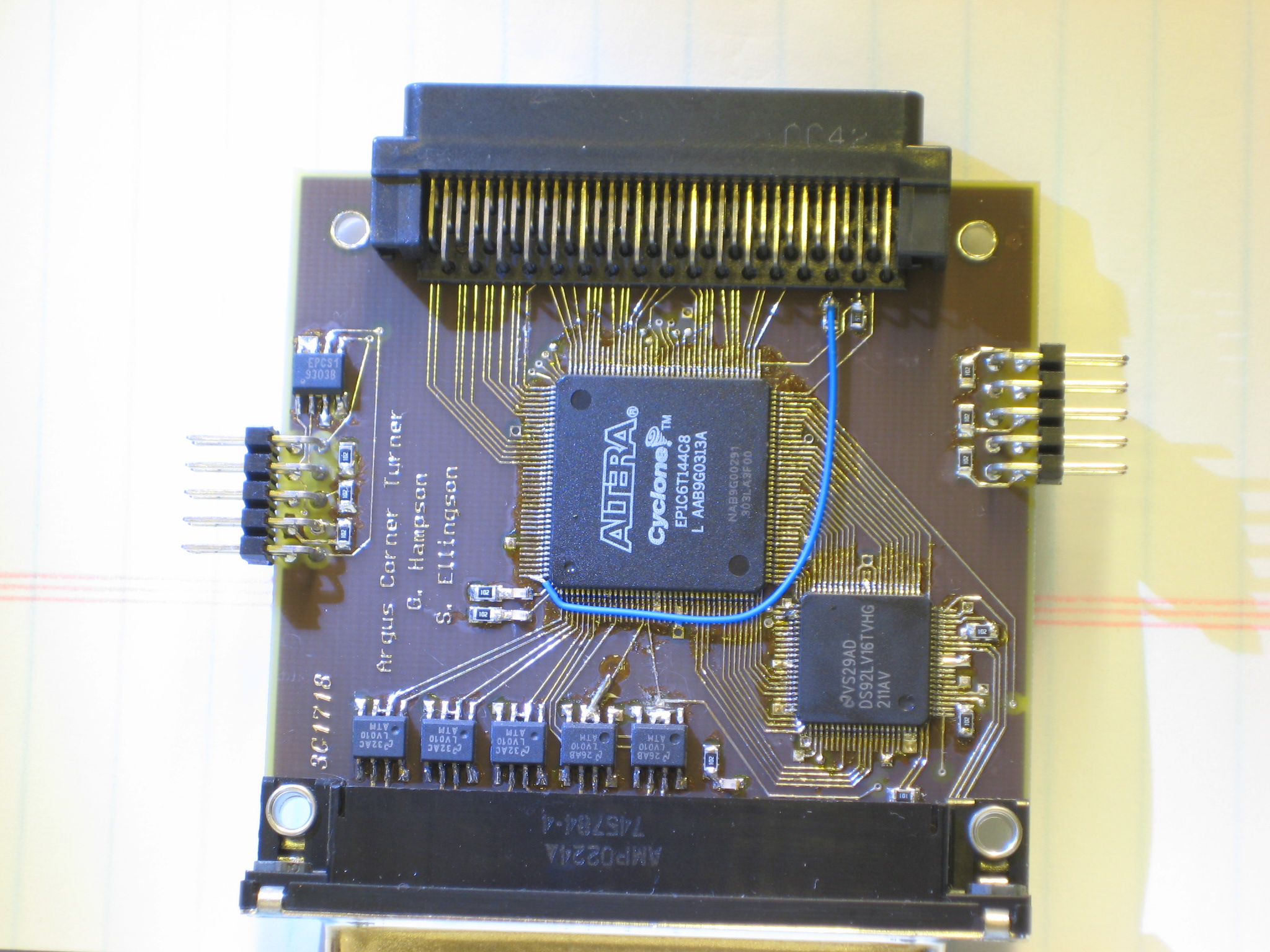
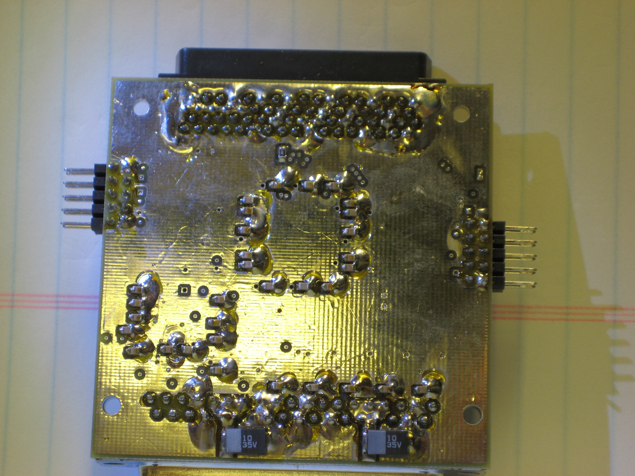
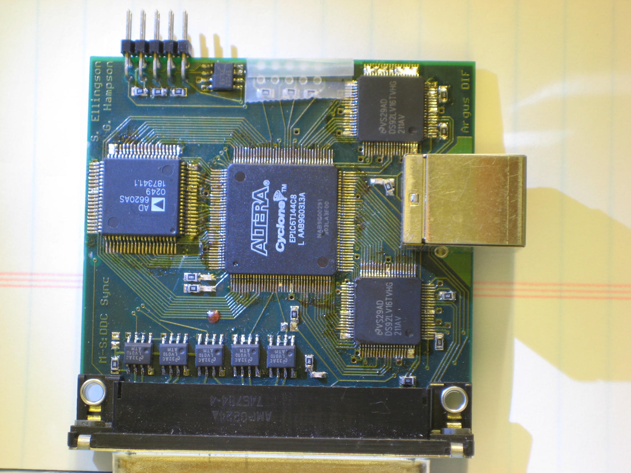
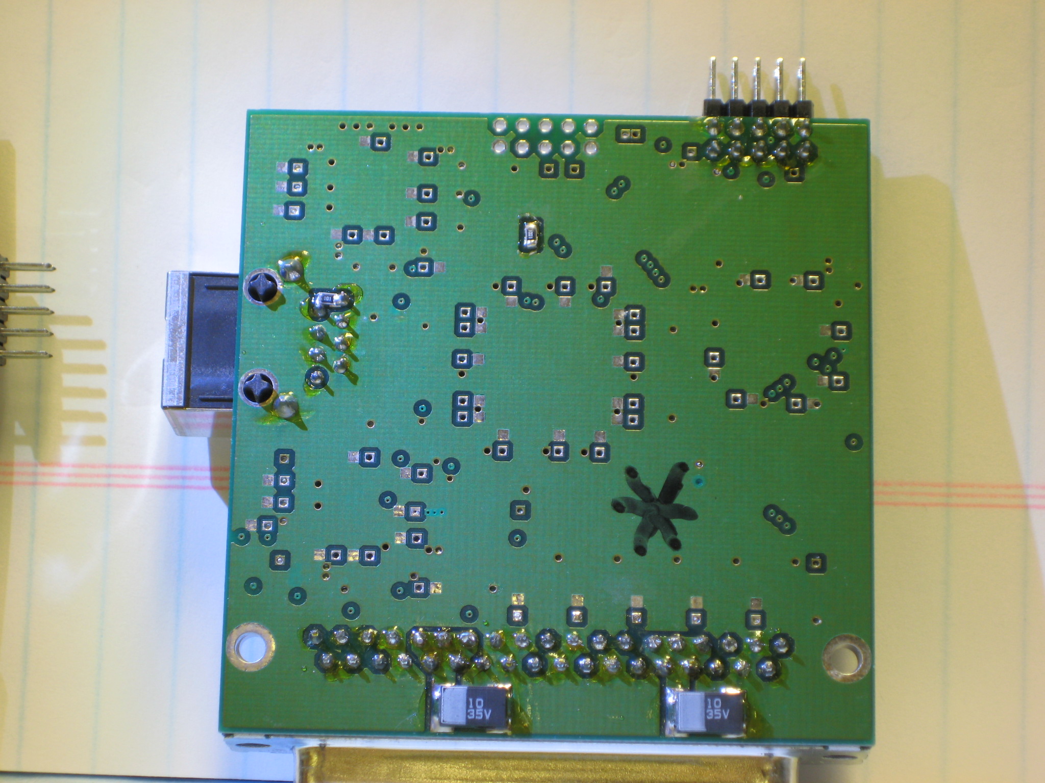
These images were taken on June 7, 2008
Corner-turner: front
Corner-turner: reverse
Normal DDC: front
Normal DDC: reverse
One of the computers crunching Argus data is tasked with looking for the broadband sources once a second, using 0.2-seconds-worth of data. The Sun shows up nicely in this integration period, provided it is above 25 degrees altitude. Satellites also show up nicely. In the above GIF animation, you can see the Sun swooping through the sky, from left to right, across the bottom half of the animation. When the sun is down, you see noise splattered across the sky.
The animation has about 17 days of the sun, without too much additional events. However, at about the 18th day, I changed the frequency of the Argus receivers and suddenly GPS satellites started showing up, in their characteristic 12-hour orbits. These are the trails which appear to be 'springing' across the sky.
The time span is speeded up so that each day takes about 2 seconds. The animation repeats without pause.
I changed the Argus frequency to 1296.000 MHz last week. Mike Murphy suggested that it would be a good test of Argus if we could try to detect the SETI League 1296 MHz moonbounce signal.
The moonbounce signal was not detected, but this frequency band is not quiet, either. There appears to be a 1296 MHz signal emitting or reflecting from satellites, causing short-term narrowband blips. These blips are relatively strong, and they make an excellent match with the "ideal beams" of the array, indicating far-field radiators.
These are definately "local" signals that we're seeing here, because the source is moving fast across the sky (about 20 degrees in 1 minute). The stars "move" at a rate of 1 degree every 4 minutes - at the fastest. Some stars like the North star, Polaris, barely moves at all.
I have created a movie of a "blip" as it occurred on May 4, 2008. The movie is put together in one-tenth-second frames, showing what the source would have looked if you had "radio eyes", only 10-times faster, for display purposes. The coordinates are not labeled on the movie, so here they are:
Left border: 230 degrees azimuth
Right border: 270 degrees azimuth
<--> 40 degrees wide
Bottom border: 25 degrees elevation
Top border: 55 degrees elevation
<--> 30 degrees high
The source started at 2008-05-04 13:24:00 UTC and was observed (on and off) for 50 seconds. The animation is ten-times faster, to enhance the satellite's movement, so the movie goes for about 5 seconds, then repeats. The frequency is approximately 1296.014 MHz.
Click on the thumbnail movie below, to see the full-size version.
Note how the source flickers as it moves from the upper-left to the
lower-right. You should be able to pause the movie with the
Angelo suggested that a "trail" might be seen, if all images in the
animation are summed. Looks like that's the case:
map_average.gif
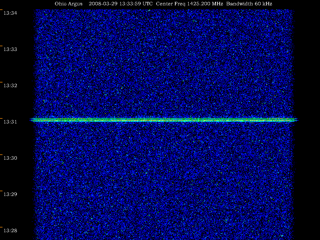
The waterfall display (color-coded intensities, frequency on the
horizontal axis and the most recent data at top) shows the flickering source
as a couple of red dots on the lower-right of the image:
wfall_20080504.png
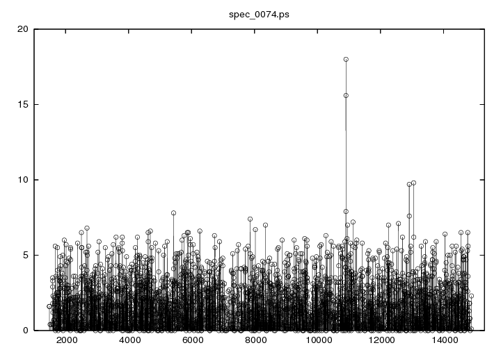
The full-bandwidth spectrum at the peak power:
spec_0074.png
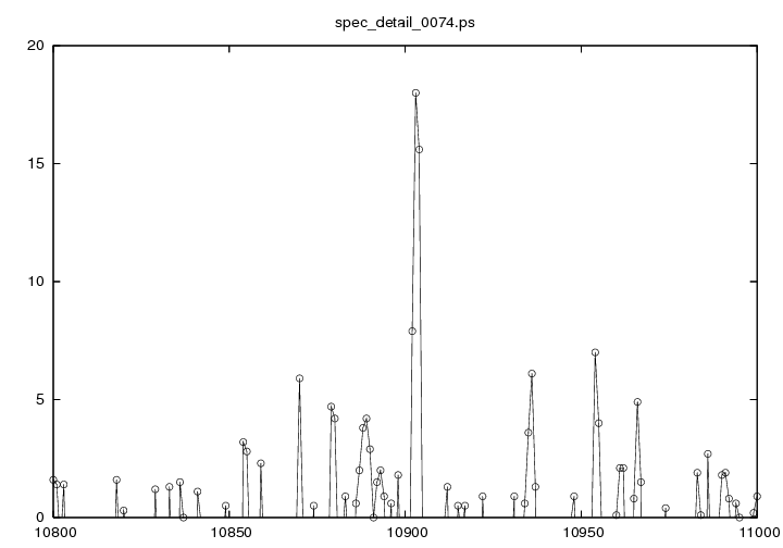
A closeup of the spectrum at the peak power:
spec_detail_0074.png
broadband_spike_20080329.png (71,797 bytes)
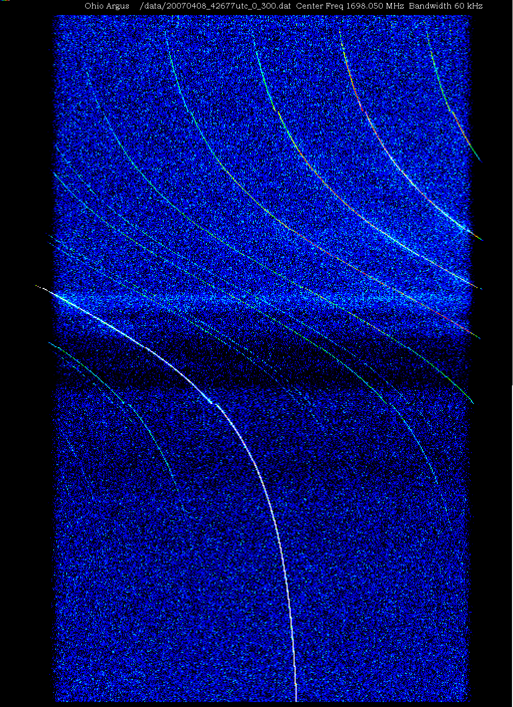
Here is a NOAA weather satellite, captured in full, on
Sunday April 8, 2007, from 11:45 UTC (bottom of image) to
11:56 UTC (top of image). [That's 15:45 - 15:56 EDT]
Center frequency is 1698.050 MHz.
Look! at the central carrier. Thrill! at the sidebands.
Stand in awe! at the doppler shift as the satellite whizzes
overhead. Scroll down! because this is a "tall" image.
sat_20070408.png (231,542 bytes)
These spectacular images happen several times a
day now. You can see them if you watch the waterfall
display
here.
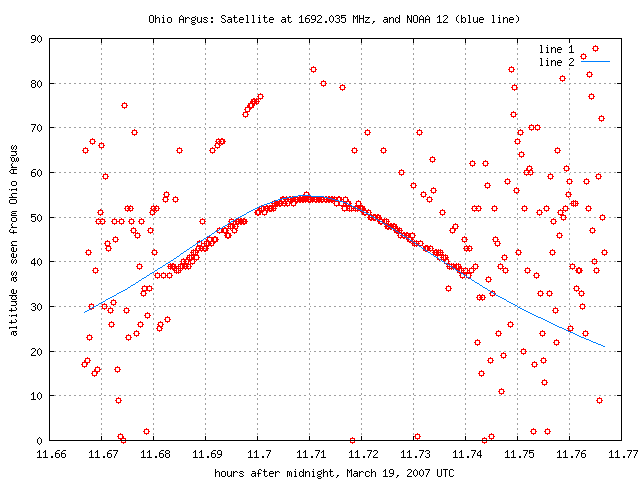
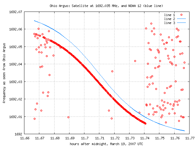
Mike Murphy has identified the satellite which we have
seen here at Argus for the past 2 1/2 years. It is
NOAA 12, a polar-orbiting satellite. Apparently, NOAA 12
broadcasts data at 1698.0 MHz, but we are seeing a "spur"
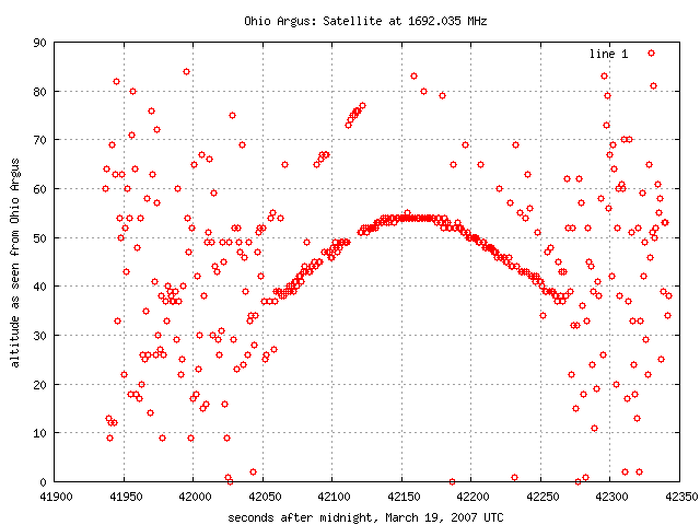
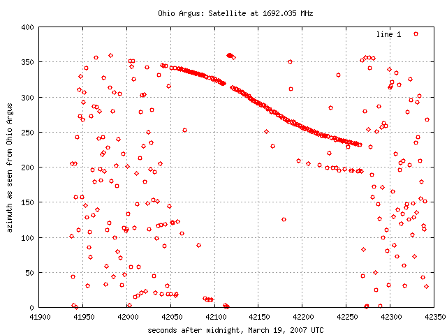
at 1692.035 MHz. Below is the same set of plots as seen in
the previous article, but this time with the orbital
data of NOAA 12 added in (blue lines).
Here is the altitude:
Here is the azimuth:
Here is the frequency:
I'm sure some of the NAAPO volunteers will take a stab
at accounting for the 5 kHz offset of the predicted
frequency.
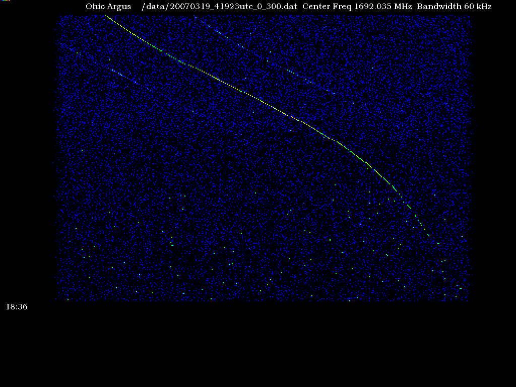
Here is a waterfall frequency spectrum of a satellite
seen by Argus on March 19, 2007, from 11:32 to 11:38 UTC.
Note the "side bands" on either side of the central signal.
The center frequency is 1692.035 MHz; bandwidth is 60 kHz.
The oldest time is at the bottom and the most recent time
is at the top. The highest frequency is at the right; the
lowest frequency is at the left.
sat_20070319.png (39107 bytes)
Here is the altitude:
Here is the azimuth:
Here is the frequency:
This satellite trace is significant only because it is the
best data seen by Argus in about 6 months, ever since
horrible-looking interference started showing up in the
narrowband data. To eliminate this interference, I
changed the "second local oscillator" frequency from 1 MHz
to 2 MHz. This may not mean a lot to most of you, but
essentially it means that there a problem with some of
the receiving equipment, and my desired setting is now
undesirable. It's like having a radio with a volume knob
that is "crackly" at a certain volume level, and you have to
turn the volume up or down slightly to get the crackle
to go away. The volume may not be exactly what you want, but
at least you can make out what is being said.
The changing of the local oscillator was a "last-ditch effort"
on my part to find the source of the interference. There was
no evidence that the interference was happening out there
in the "real world", so I tried "turning the knob". (More accurately,
there are many "last-ditch efforts" employed in finding the
cause of problems like this. Oftentimes "remedies" come
like a bolt of lightning in the middle of the night. This
time, however, the remedy was an "oh, what the heck, I'll
try it" one.)
Continuum data collected from 1993 through 1997 is now
available to the world. I have arranged the data
by "Hour of Right Ascension". Images are in small and
large sizes, for those with low or high screen resolutions.
Small images:
https://ohioargus.org/~rchilders/contin/html_small/contin_small.html
Large images:
https://ohioargus.org/~rchilders/contin/html_large/contin_large.html
Click on one of the links above, then click on "Top declination of RA hour 00".
You will see the first declination of the survey (+62 degrees 20 minutes declination).
This data was collected in September/October 1993.
There were three days' worth of data taken at this declination, hence
you see three traces. There is a nice, low-power point-source which passed
through the "leading beam" at around point 295, and through the "trailing beam"
at around point 330. These "points" correspond to 10-second samples. Thus,
point sources at this declination show up ~35 samples, or 350 seconds,
from beam-to-beam. This spacing drops to 150 seconds at 0 degrees 0 minutes
declination.
The reason why I point out the beam-to-beam spacing is because "one beam" radio
telescopes (the vast majority) have trouble telling the difference between noise and true sources,
unless they have several days' worth of data. A "blip" may be a celestial source
or terrestrial noise. But with Big Ear's "dual beam" setup, celestial sources
make characteristic "dual-humped" patterns. This dual beam is a blessing and a
curse, however, because if two sources are closer than the "beam spacing" they
will interfere with each other. Also, any diffuse background sources (eg
the cosmic microwave background) is completely hidden in this dual-beam paradigm.
But dual-beam observing gives quick "confirmation" that a celestial source
was seen, and a simple deconvolution algorithm can transform dual-beam data
into single-beam data (with the exception of diffuse background sources).
Three comments on the collection of images: (1) There are 540 data points in
each image, corresponding to 5400 seconds of observation "per hour". "But Russ,"
you say, "there are only 3600 seconds in an hour." You are correct. The images
I've generated actually start 15 minutes (900 seconds) BEFORE the hour, and end
15 minutes (900 seconds) AFTER the hour. 3600 + 900 + 900 = 5400 seconds. I did
this so sources which fall at the "top of the hour" do not get "clipped". Thus, the
"top of the hour" starts at sample 90, and the hour ends at sample 450. (2)
The "first" declination shown is always +62 d 20 m. Click on the "lower" hyperlink
to go to the next-lower declination: +62 d 00 m. All declinations are separated
by 20 minutes of declination (1/3 degree). The lowest declination is -36 d 40 m,
and was taken at the end of August, 1997. The astute observer will see sources
get "brighter", and then "fade" with passing declinations. Declination -16 d 00 m
is the only one "missing", and I will try to find out what happened to that data.
(3) The sun passes through the beams even when the
beams do not point directly at it. You will recognize the sun, because (a) it
shows up in later-and-later locations in each days' data, and (b) it is broad, and
makes a characteristic "large-angular-extent" dual-beam pattern, unlike the
weak point-source example above. The moon also shows up occasionally. See if you
can spot it. (Hint: it should only show up between declinations +28 and -28 degrees.)
Also, "sun dogs" appear before and after the sun when the sun passes through the
beams.
Now to the meat of the matter. Sources which show up day after day are nice to
know about, but the real exciting sources are the ones which pop up only
occasionally. Suppose the "weak point source" illustrated above only showed up
on one of the traces. That would be VERY interesting. Now suppose that source
appeared in the "leading beam" on one day and in the "trailing beam" on another
day. That would be VERY VERY interesting. Bob Dixon has claimed that "if you
found a source like this, you would be instantly famous".
A note to those who wish to be famous: I have looked for "spikes" in the
data, corresponding to these VERY VERY interesting sources. I have come across
many more "positive-going" spikes than "negative-going" ones. This indicates
that there is some local interference causing biased spiking, because if the
spiking sources are truly celestial, then there would be - on average - the
same number of positive- as negative-going spikes.
A note to those who wish for near-fame: Sources which show up in each
beam on each day may not be as boring as I allude to above, IF THEY
DO NOT SHOW UP WITH THE SAME POWER IN THE ORIGINAL OHIO SURVEY. A source
in the Ohio Survey may be much brighter in the 1993-1997 survey, or may
have gone away. Either way, a source-by-source comparison should be made
with the original Ohio Survey.
A note for you techie astronomers out there. The "declination" is
the "declination at the epoch of observation" and has not been precessed
to another epoch. Similarly, the "Right Ascension" is the "Local Mean Sidereal
Time" and has also not been precessed to another epoch. The Ohio Survey source
catalog and contour maps were precessed to epoch 1950.0, and so source-to-source
comparisons of the 1993-1997 data and the Ohio Survey catalogs is "tricky".
One last note. A couple of times the data collection computer's clock differed
from the true time (UTC) by as much as a minute. This shows up in the images
as sources which appear shifted in time from their counterparts. No attempt has
been made to correct these clock errors, however I carefully noted these clock
anomalies in several log books when I encountered them at the time.
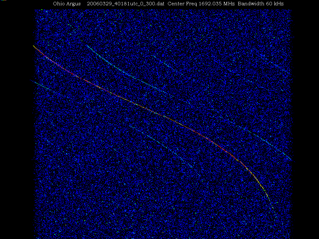
After observing the radio band at 1420.470 MHz over the winter,
horrible interference and a desire for greener pastures
has driven me to tune Argus back to 1692.035 MHz, where
satellites abound. Click
here
for an awesome satellite trace, observed on March 29, 2006.
I spoke above of "horrible interference" at 1420 MHz. I was
surprised to find this interference, because 1420 MHz is supposed
to be "protected" for radio astronomy. Oh well. I am also
disappointed that Argus was unable to locate the source of
the interference: Argus specializes in locating sources with
arbitrary locations.
Interference screen capture #1.
Interference screen capture #2.
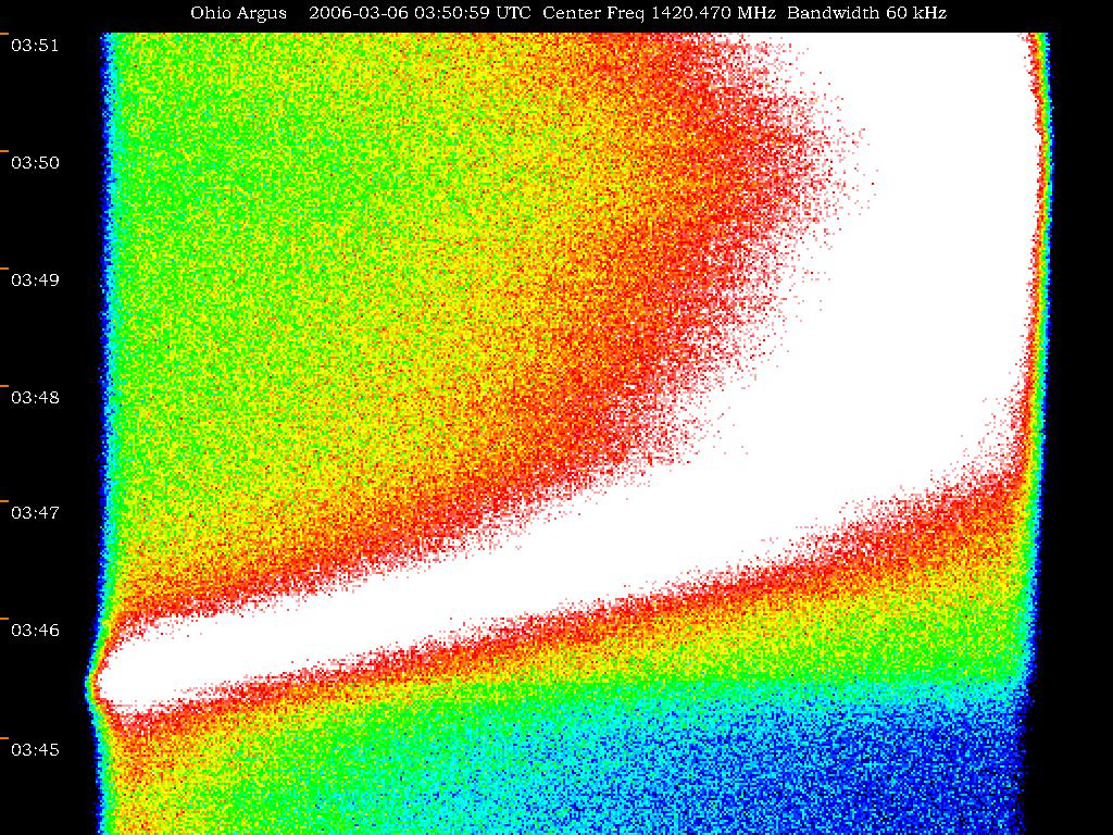
When doing radio astronomy, it is essential to have on hand
a calibration source, which lets the observer know that the
equipment is functioning properly. Radio astronomers will
often use a "noise source" to do this calibration at regular
intervals. The Ohio Argus Array uses such a noise source, which turns
on for one second, once per minute, 24 hours a day. The parabolic
dish at SatComm does not have such a calibration (yet), so instead
I have used my hand to calibrate the parabolic dish feed. I have
found that when my hand is in front of the feed, the power output
of the receiver system rises by 3 dB, or by 2-times the normal
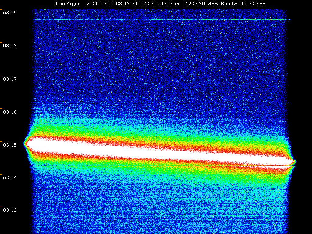
output. Here
is a waterfall snapshot of my hand in front of the
parabola's feed for about 30 seconds (the light blue stripe at the center
of the image). The total time in the
waterfall image is 5 minutes, with the most recent time at the
top. Frequency goes from lowest at the left to highest at the
right. The center frequency is 1420.470 Mhz, and the bandwidth
is 60 kHz. (Ignore the 00:55 at the lower left - it is a data
processing artifact.)
The real-time waterfall output from the dish is now available online
at this URL:
https://ohioargus.org/Argus/data/display2.html. Note that the
top of the waterfall says "Argus Dish", and the page is named
"SatComm Parabolic Dish Waterfall Display". This is not to be
confused with the real-time Argus Array output here:
https://ohioargus.org/Argus/data/display.html.
Note that the
top of the latter waterfall says "Ohio Argus", and the page is named
"Ohio Argus Waterfall Display".
The astute observer will also note that there is
just over 6 minutes of data on the "Argus Dish" page, whereas there
is 6.5 minutes of data on the "Ohio Argus" page. This is because
the spectra with "calibration on" have been excised from the
"Ohio Argus" page; there is no regular calibration on the
"Argus Dish" page: all those spectra have been left in. Since both
displays show the same number of spectra per image, the time
stamp of the oldest data on the "Ohio Argus" page will be older
than that on the "Argus Dish" page.
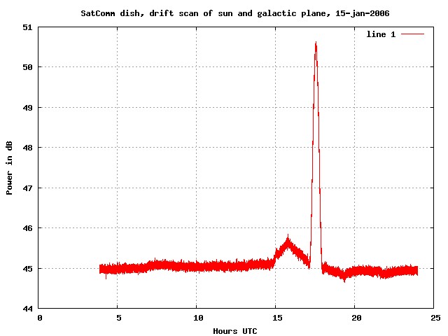
Here is a meridian drift scan of the sun and galactic plane
through the main beam of the 10-foot parabolic dish at
SatComm on January 15, 2006. The declination of the dish is
roughly -20 degrees. The center frequency is 1420.470 MHz and
the bandwidth is 60 kHz. Each data point is the total power,
in dB, of 16384 samples taken over 0.205 seconds. Data points
are one second apart. No averaging across data points is done.
The galactic plane is seen at about 16 hours UTC, and the sun is
at about 17.5 hours UTC. The Galactic Center is located at -29
degrees declination, so the beam is rather close to the "brightest"
part of the galactic plane (see this
image of the radio sky from Kraus's
Radio Astronomy). The half-power beamwidth of the 10-foot
parabola at 1420 MHz appears to be about 5.5 degrees, after taking
the apparent width of the sun (0.5 degrees) and the declination of
observation into consideration.
sun_and_gp_20060115.jpeg (96596 bytes)
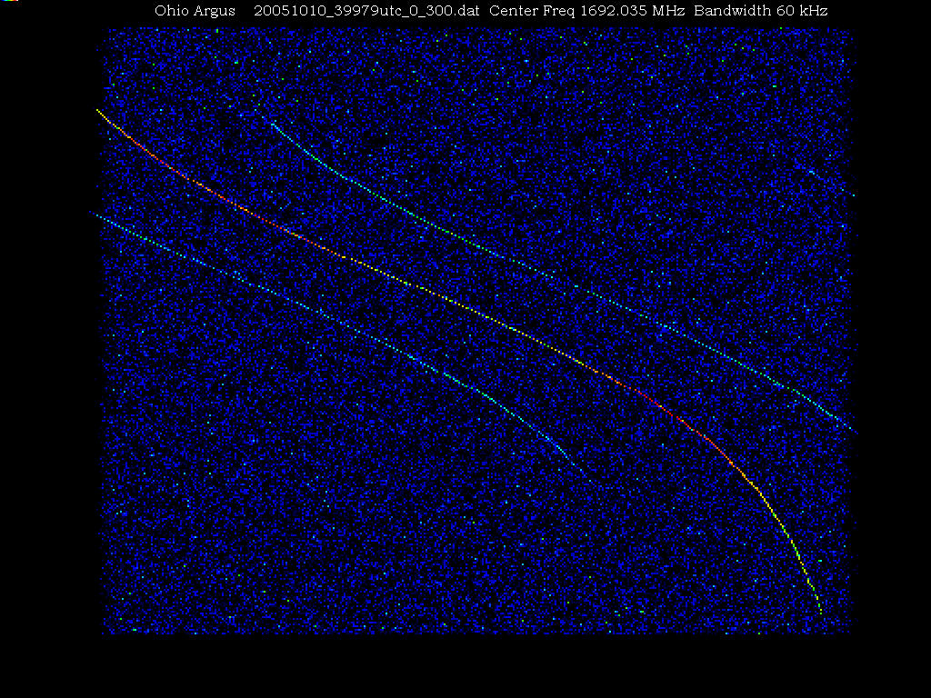
Here is a waterfall frequency spectrum of a satellite
seen by Argus on October 10, 2005, from 11:02 to 11:05 UTC.
Note the "side bands" on either side of the central signal.
The center frequency is 1692.035 MHz; bandwidth is 60 kHz.
The oldest time is at the bottom and the most recent time
is at the top. The highest frequency is at the right; the
lowest frequency is at the left.
The S-shaped frequency profile suggests
that this is a low-earth-orbit satellite, where the frequency
goes from high to low, like the sound of a race car's
engine as it passes you on its way around the track. The intensity
of the signal goes from low (green) to medium (yellow) to high (red),
and then back down to low.
spectrum_20051010.jpg (298299 bytes)
Below is a polar plot of the above satellite.
The image represents the sky as an observer on the ground would
see it. The circle is the horizon; the top is North; West is on the
right; East is on the left; South is on the bottom. The point
"directly overhead" is in the center of the circle. The satellite
track goes from close to the North horizon, to near overhead, to slightly
south. This plot shows the location only of the satellite, not the
frequency or intensity, which are both seen in the above waterfall image.
Points (*) not on the track are either noise, or sidelobes (false
location) of the satellite's location.
skytrackB_20051010.jpg (60329 bytes)
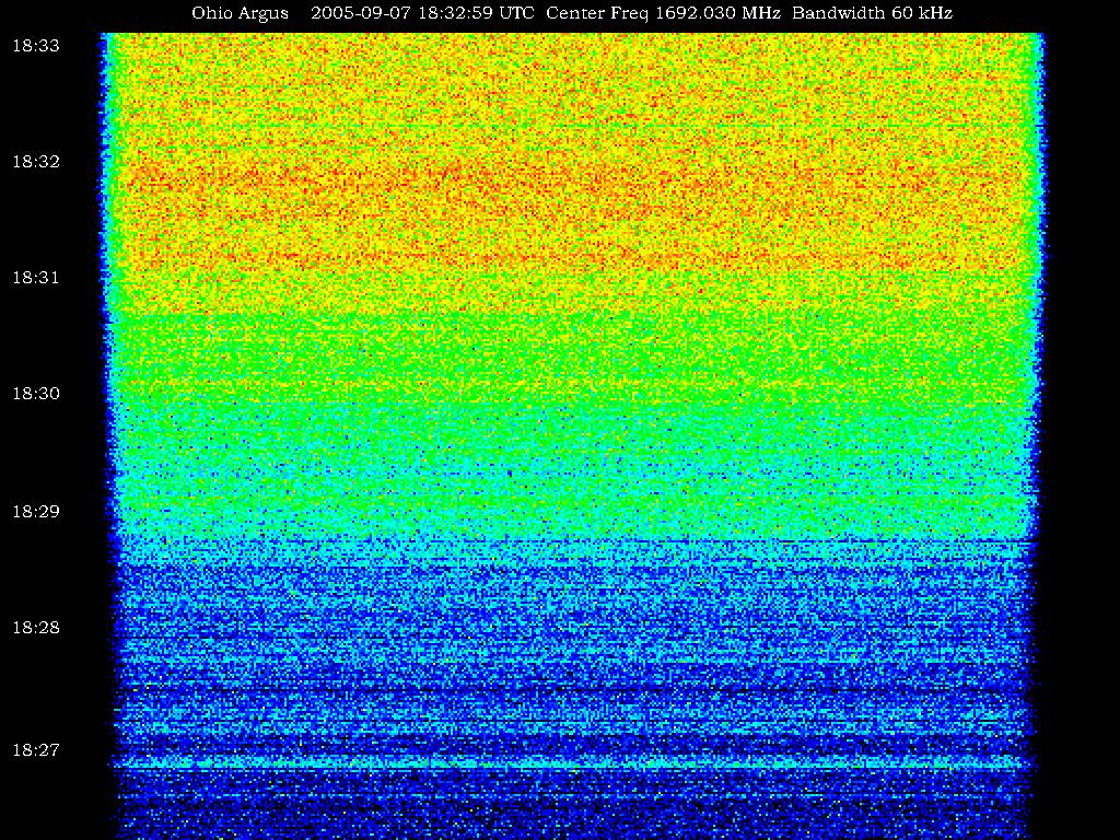
Here is a screen capture from the Argus waterfall:
outburst_20050907.jpg (318684 bytes)
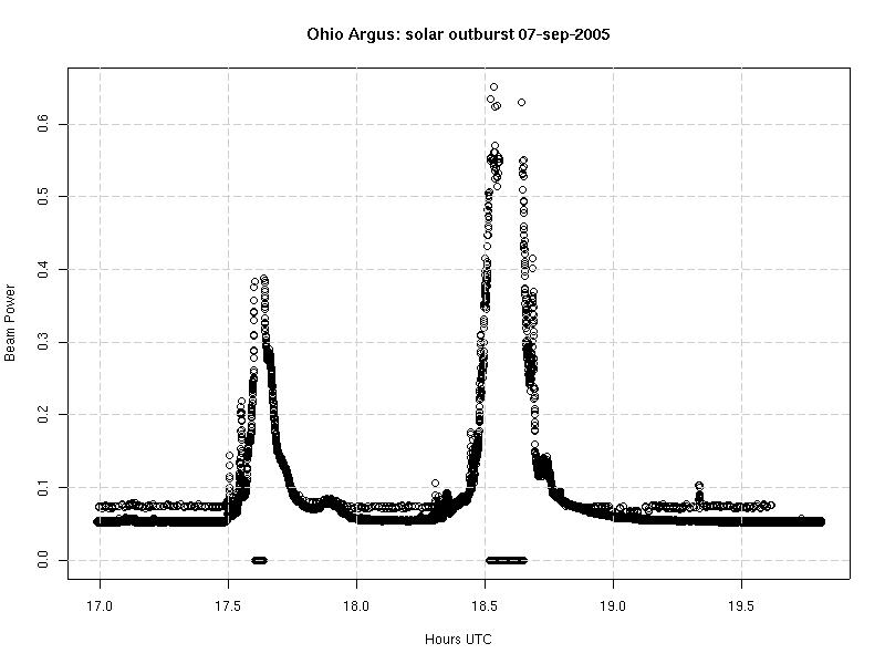
...and here is a plot of "beam power" for a three-hour time period:
outburst_plot_20050907.jpg (49393 bytes)
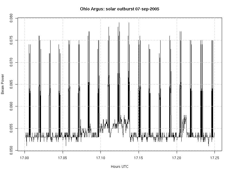
...and here is a closeup of 15 minutes from 1700 to 1715 UTC. I don't know
if the sets of spikes are local interference or are part of the solar
outburst. The spikes were not caused by the calibration source, because
the calibration source fired for one second each minute, and these spikes
fired in groups of three or four 19 times in 15 minutes.
outburst_plot_20050907.jpg (65583 bytes)
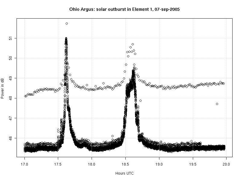
This burst was so powerful, it showed up in all Argus elements, and in fact saturated
most of them. Below is the power seen in Element #1 for the 3 hours around the
outburst. Recall that the elements have roughly hemispherical coverage, which is
a heck of a lot of square degrees. The sun covers a tiny part of the sky, and the
outburst was a tiny part of the sun. The burst must have been VERY powerful to
actually show up in individual elements. The calibration source is seen floating
between 48 and 49 dB.
outburst_elem1.jpg (59764 bytes)
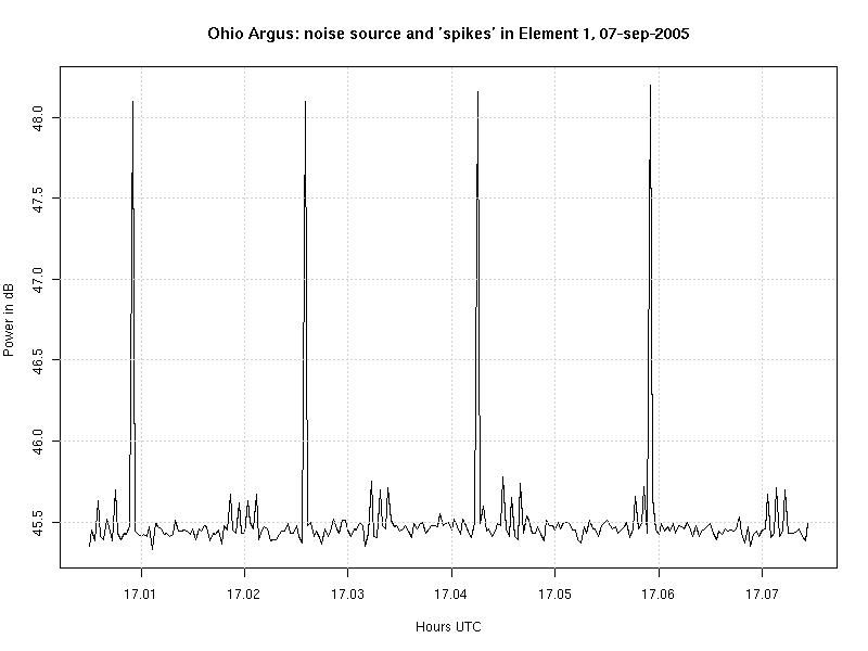
The following graph is a closeup of the above graph from 1700 to 1705 UTC.
Note the noise source every minute up around 48 dB. Also note the six
groups of spikes between 45.5 and 45.7 dB.
outburst_elem1_closeup.jpg (45799 bytes)
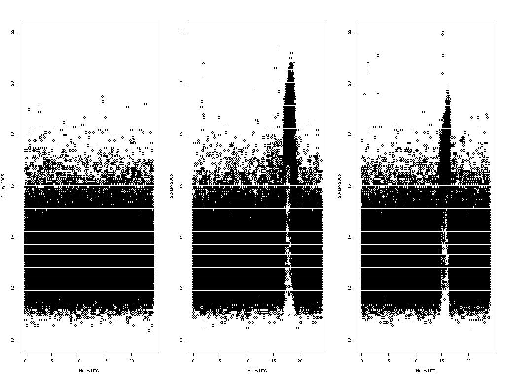
The sun generated two several-hour-long flareups, as observed at 1692 MHz,
at 18 hours UTC on August 22, 2005, and at 15 hours UTC on
August 23, 2005. The following plots show data from August 21,
for comparison, and from August 22 and 23.
The first plots show the "best beam" power as seen by Argus in its entire
60 kHz bandwidth. The "best beam" points at the sun during mid-day. The sun
reaches its highest altitude, and strongest power, at around 17:30 hours
at Argus's longitude. Note the low hump in the August 21 plot, and
the high peak around 18:00 on the 22nd and around 15:00 on the 23rd.
(The data is not smoothed; power is in "dB"; artifacts are not removed;
power is sometimes "negative", because the "best beam" power is subtracted
from a reference beam, which is occasionally stronger.)
best_beam_outburst.jpg (68311 bytes)
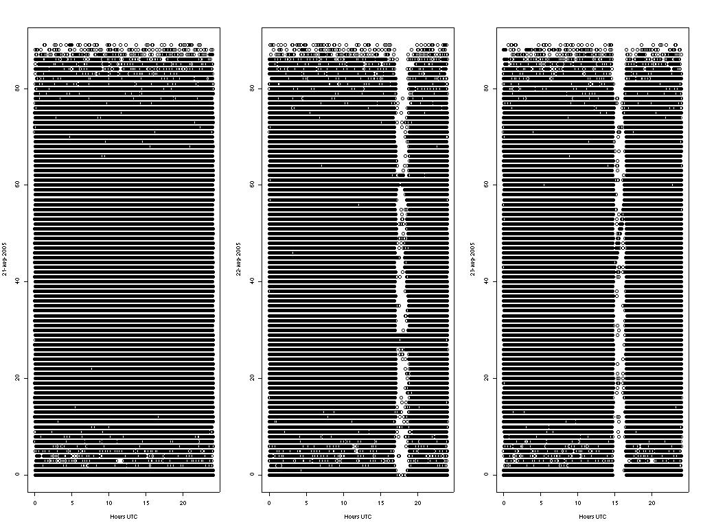
The next plots show the "best match" which a 1.5 millisecond (128-snapshot)
acquisition made to an "ideal" Argus beam. Argus was using 23 elements in
its array on these observation dates, so the "best match" is ideally
23 out of 23 element phases. Random noise will produce 23/2 = 11.5
out of 23 element phases. I show here the 128-snapshot acquisitions
instead of the full 16384-snapshot acquisitions, because the sun ALWAYS
produces a "best match" of 20-22 element phases when it is high in the
sky in the 16384-snapshot acquisitions (essentially a longer integration
time). As you can see below, the number of elements which made the "best
match" on August 21 was a random value centered on 13 element phases. But
on August 22 the best match peaked at 21 at 18:00, and on the 23 the best
match peaked at 20 at 15:00.
best_match_outburst.jpg (141081 bytes)
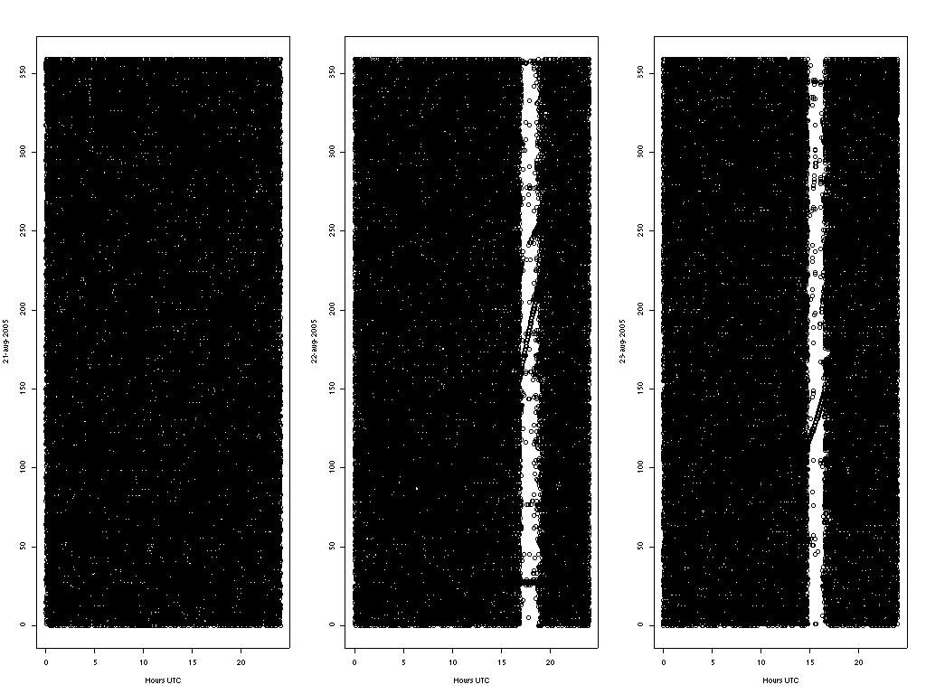
The next two plots show the altitude and azimuth of the "best match" for
August 21-23. The altitude and azimuth are simply the alt/az of the
ideal beam which the "best beam" was pointing at. On the 21st the alt/az
are just random values spaced between 0-90 and 0-360 degrees respectively.
However, on the 22nd, the altitude lingers around 62 degrees and the azimuth
goes from 160 to 210 degrees. On the 23rd, the altitude goes from 45 to
55 degrees, and the azimuth goes from 110 to 150 degrees. These alt/az
ranges correspond to the the motion of the sun for several hours around
18 hours UTC on the 22nd and for several hours around 15 hours UTC on the 23rd.
best_alt_outburst.jpg (190673 bytes)
best_az_outburst.jpg (130884 bytes)
Note: The sun was also seen in the strongest 5-Hz bins, and was accurately
located in altitude and azimuth, even though the outburst was spectrally
flat in the 60 kHz observation bandwidth. This provided a confirmation that the
narrowband source algorithm (which uses FFTs as data) can also provide
accurate pointing information. (Narrowband data not shown).
In preparation for attempting to observe Cas A, I observed the
sun on August 10, 2005 as it transited the meridian. The data for the plot
below consists of data points taken at one-second intervals.
Each one-second point is actually 0.2 seconds of data captured
in 16,384 analog data points, with each data point squared,
summed across all 16,384 points, and then divided by 16,384.
The resultant data point is 10*log10 of the mean-squared value.
https://ohioargus.org/Argus/data/display.html
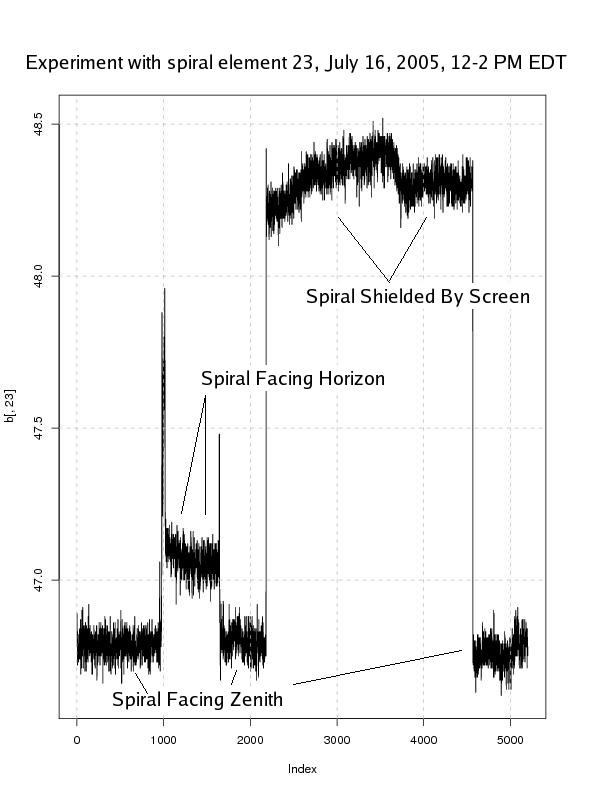
I tried to determine if an element reported different powers when
pointed toward the sun, vs pointing away from the sun. This experiment was
conducted when the sun was close to the meridian, at about 72 degrees
altitude.
The plot of data generated during this experiment (see below) is
the power in dB. (Sampled data, with zero DC component,
sum of 16384 squared samples divided by 16384; 10*log10(sum).)
A) Samples 1 -> 1000 are with the spiral "pointed at zenith".
From the graph, the lowest power was with the spiral pointed at zenith,
with the sun "in the main beam" (A,C,E). The spiral "edge-on to the sun" (B) produced
higher power because it was seeing the "hot" roof of SatComm (I suspect) in half
of its main beam. The highest power was when the shielded screen covered the spiral (D),
because a "hot" object filled the entire "main beam" (I suspect).
This impressive
source is seen as it goes from alt 30, az 10 degrees, through zenith, and
ends at 30 alt, 200 degrees azimuth. The main signal starts at the right-hand side of the
screen, and ends at the left-hand side. The S-shape is caused by a change in
Doppler shift of the signal: there is less Doppler shift in the rising and setting
as compared to when the source is overhead (think of the sound of a race car
as it zooms past a spectator close to the track). The sidebands follow the
shape of the main signal. The center frequency is 1692.030 MHz, with a bandwidth
of 70 kHz. The entire screen is about 8 minutes in time.
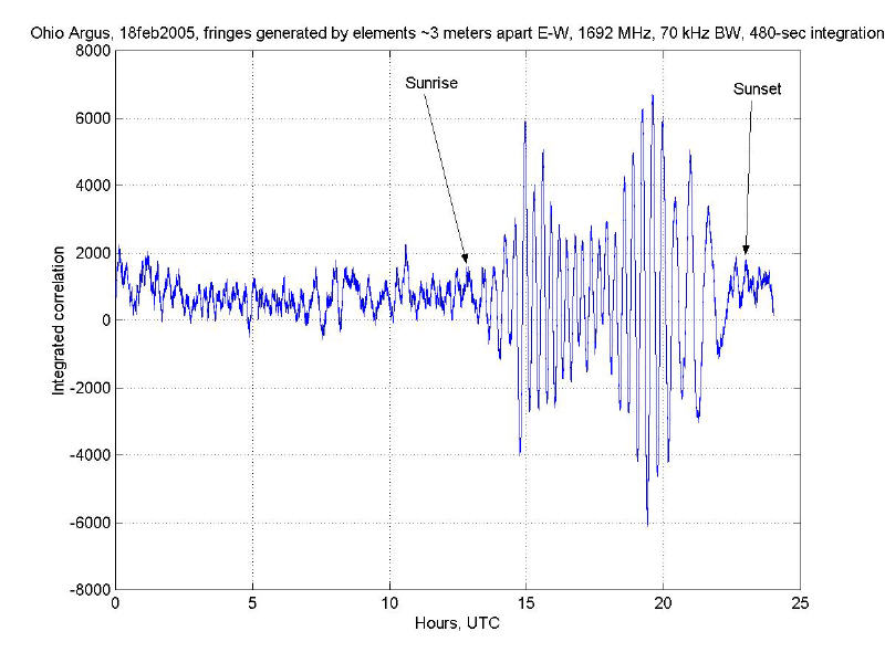
The sun as seen by Argus on February 18, 2005. This image was generated
in "interferometry" mode, using two elements approximately 3 meters apart,
roughly on an east-west line. Data was generated by multiplying each
elements' I-value and summing, and multiplying each elements' Q-value and
summing. A 400-acquisition moving window convolution was done over the
entire 24-hour set of acquisitions, resulting in a "480-second" integration
time. The x-axis is the UTC time; the y-axis is the sum of correlations
centered on the 400-acquisition window. Note the interferometric "fringes"
while the sun is above the horizon. Fainter fringes might be seen when
the sun is below the horizon, perhaps caused by the Cas A supernova.
Receiver center frequency is 1692.030 MHz; bandwidth is 70 kHz; each acquisition
takes 0.2 seconds; there are 16384 samples per acquisition; time between
acquisitions is 1.2 seconds.
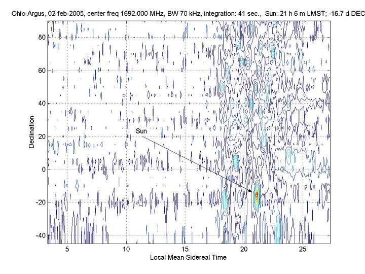
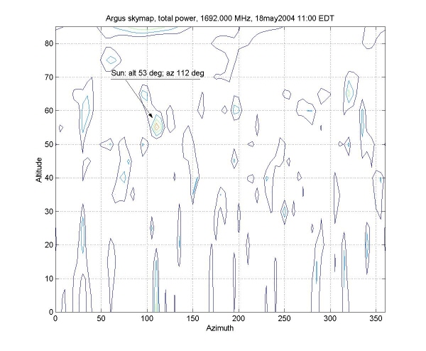
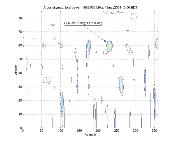
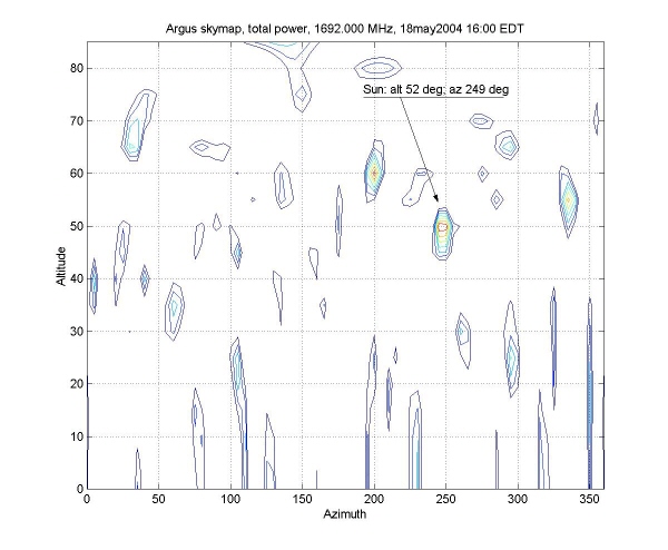
The sun as seen by Argus on February 2, 2005. This image was generated
by combining many "drift scan" beams into one contour plot. The drift scan
beams are aligned along the meridian, at 5-degree altitude intervals.
Center frequency is 1692.0 MHz, bandwidth is 70 kHz. Integration time
is 41 seconds, which is derived from averaging 200 0.205-second acquisitions.
The x-axis is hours of Local Mean Sidereal Time. The y-axis is degrees of
declination. Sidelobes of the sun appear at various locations. These sidelobes
all appeared on the meridian, because that's where the beams were pointed.
Note the sidelobes close to 90-degrees declination. One would expect these
sidelobes to be smeared out, because the plot is a "mercator projection".
But this is not the case, because sidelobes can travel fast through the pole.
There is no indication of Cass A or Sgr A (bright extra-solar sources), but
this is not unexpected, because these sources passed through the meridian
while the sun was up.
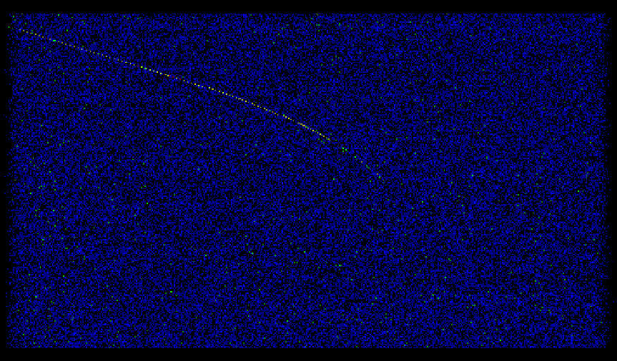
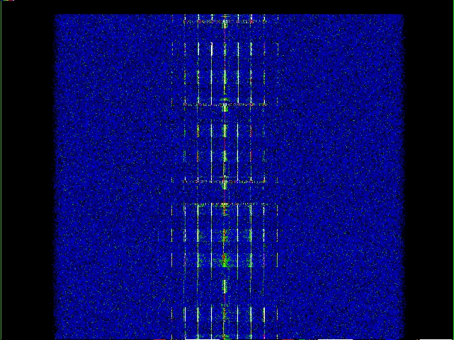
This source
was seen by all who attended the radobs meeting on
Saturday, October 2, 2004. Argus
formed beams all over the sky, searched for the
strongest narrowband source in each beam, then
used the spectrum of the "strongest" beam to create
the waterfall. The source appears to be a satellite
going directly overhead from north to south along the
meridian. The source shows up in the center of the screen,
at alt/az 45/10, and ends up on the left-hand side of the
screen at alt/az 80/200. Center frequency is 1692.030 MHz,
with a bandwidth of 70 kHz. The time of the bottom spectrum
is 10:07 EDT and the top spectrum was taken at 10:13 EDT.
nb02oct2004_5.jpg (213159 bytes)
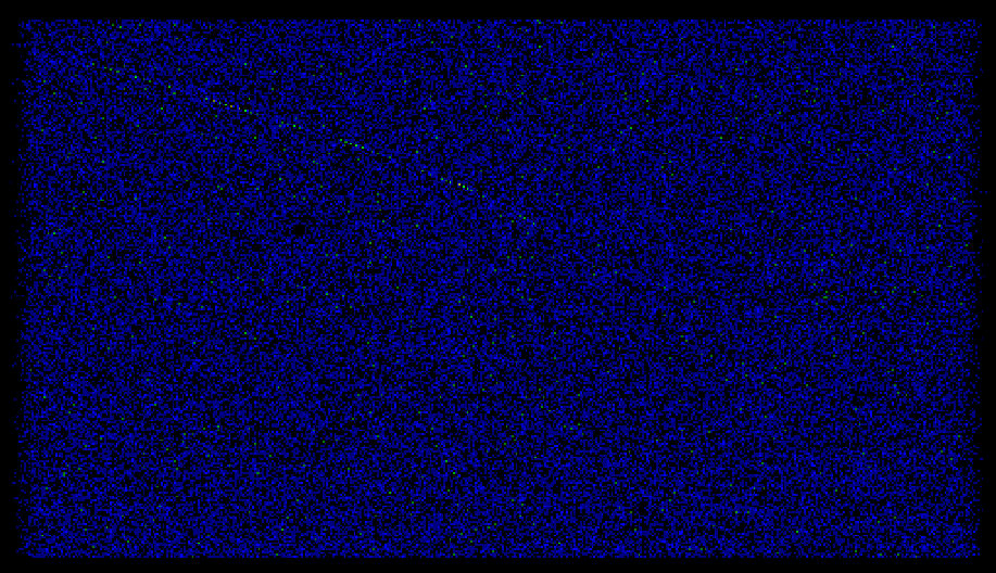
The same narrowband source as above, except Argus
has a "fixed" beam at alt/az 43/168. Note that without
tracking, the signal seems to be weaker and fades in and out.
This is because the source is passing through sidelobes of the
43/168 beam.
nb02oct2004b.jpg (231451 bytes)
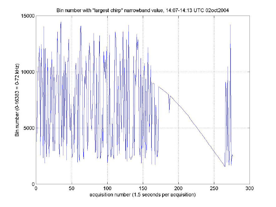
A plot of the "best" narrowband frequency for the "tracked
source" above. Note the smooth curve in the middle of the plot.
This curve, combined with alt/az data could allow us to determine
the orbit of the (supposed) satellite. It is not known, however,
if the received 1692 MHz signal is steady, or if it originates
from the satellite, or if it is a reflection from some other
source. The x-axis is the 1.5-second acquisition number, and the
y-axis is the "frequency bin" number (bin 0 -> 16383 =
1691.994 MHz -> 1692.066 MHz).
Acquired Saturday, August
7, 2004. The beam was switching during the 10-minute
acquisition: the beam pointed at GOES (alt 43, az 168) for
40 seconds, then the beam pointed at the meridian (alt 70,
az 180). One can see the strength of the signal increase
in the GOES beam and decrease in the meridian beam.
Source frequency is 1692.0202 MHz, bandwidth is 25 Hz,
altitude is ~49 degrees, azimuth is ~110 degrees.
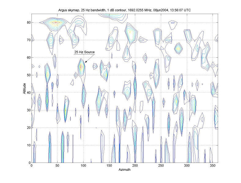
Argus sees a satellite at 13:56:07 UTC (note change from
13:55:33 on image), on 08-JUN-2004.
Source frequency is 1692.0255 MHz, bandwidth is 25 Hz,
altitude is ~55 degrees, azimuth is ~93 degrees.
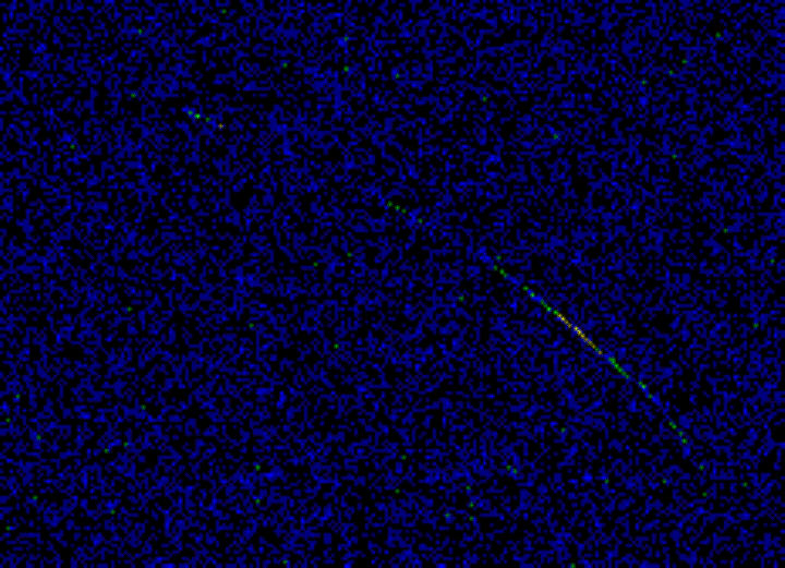
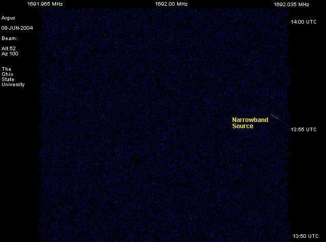
A waterfall representation of the above satellite.
The beam is pointing at 52 degrees altitude,
100 degrees azimuth (about the middle of the observed
path of the satellite). In the center-right of the
screen, the sattelite can be seen changing in frequency
over time (chirping). The chirping from high to
low frequency, combined with the rapid change in location
(shown above), is characteristic of a low-earth orbiting
satellite. The radio signal may be emanating from the
satellite, or it may be a reflection of a terrestrial
transmitter.
Each frequency "bin" is 5 Hz wide. Note that the source is about 10 Hz wide.
Broadband emission from over-flying object, March 29, 2008
Awesome Satellite Image!!!, April 8, 2007
Satellite identified, March 19, 2007
Satellite detection, March 19, 2007
Big Ear Continuum Data Browser
Awesome satellite with sidebands: March 29, 2006
Waterfall Output of Parabolic Dish: February 9, 2006
Sun and Galactic Plane Drift Scan: January 15, 2006
Satellite track, October 10, 2005
Sun outburst on September 7, 2005
Sun outbursts, August 22nd and 23rd, 2005
Sun transit as seen in 10-foot dish with Argus element as feed
Real-time waterfall display:
An experiment with Element 23, July 16, 2005, 12-2 PM, EDT
B) Samples 1000 -> 1600 are with the spiral "edge-on to the sun".
C) Samples 1600 -> 2200 are with the spiral "pointed at zenith".
D) Samples 2200 -> 4600 are with the spiral "pointed at zenith", with a
screen shielding the spiral. The screen was shielded by a non-conducting insulator.
E) Samples 4600 -> 5200 are with the spiral "pointed at zenith".
A narrowband source, with sidebands, captured May 5, 2005.
Argus sees the sun, part 3.
Argus sees the sun, part 2.
A narrowband source "tracked" by Argus.
A narrowband source caught in a waterfall beam
pointing at alt 43 deg, az 168 deg. Center frequency
is 1692.000 MHz. Acquisition time was September 3, 2004,
14:22 UTC.
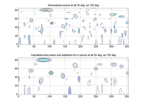
A narrowband source at alt 50 deg, az 105 deg. All-sky image
of actual data in top plot. Calculated all-sky image using
simulated data in bottom plot. Note that the sidelobes in
the top plot match the sidelobes in the bottom plot.
GOES 12 signal at 1691.000 MHz.
Argus sees a satellite at 13:55:33 UTC, on 08-JUN-2004
Argus sees the sun
 (1,548,422 bytes)
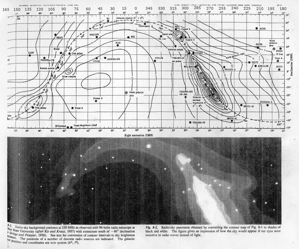